Plane poiseuelle flow solved by finite difference
September 30, 2011 at 01:05 PM | categories: odes | View Comments
Contents
- Plane poiseuelle flow solved by finite difference
- we define function handles for each term in the BVP.
- define the boundary conditions
- define discretization
- No user modification required below here
- now we populate the A-matrix and b vector elements
- solve the equations A*y = b for Y
- construct the solution
- plot the numerical solution
Plane poiseuelle flow solved by finite difference
John Kitchin
http://www.physics.arizona.edu/~restrepo/475B/Notes/source/node24.html
solve a linear boundary value problem of the form: y'' = p(x)y' + q(x)y + r(x) with boundary conditions y(x1) = alpha and y(x2) = beta.
For this example, we resolve the plane poiseuille flow problem we previously solved in Post 878 with the builtin solver bvp5c, and in Post 1036 by the shooting method. An advantage of the approach we use here is we do not have to rewrite the second order ODE as a set of coupled first order ODEs, nor do we have to provide guesses for the solution.
we want to solve u'' = 1/mu*DPDX with u(0)=0 and u(0.1)=0. for this problem we let the plate separation be d=0.1, the viscosity  , and
, and  .
.
clc; close all; clear all;
we define function handles for each term in the BVP.
we use the notation for y'' = p(x)y' + q(x)y + r(x)
p = @(x) 0;
q = @(x) 0;
r = @(x) -100;
define the boundary conditions
we use the notation y(x1) = alpha and y(x2) = beta
x1 = 0; alpha = 0;
x2 = 0.1; beta = 0;
define discretization
here we define the number of intervals to discretize the x-range over. You may need to increase this number until you see your solution no longer depends on the number of discretized points.
npoints = 10;
No user modification required below here
Below here is just the algorithm for solving the finite difference problem. To solve another kind of linear BVP, just modify the variables above according to your problem.
The idea behind the finite difference method is to approximate the derivatives by finite differences on a grid. See here for details. By discretizing the ODE, we arrive at a set of linear algebra equations of the form  , where
  and
and  are defined as follows.


To solve our problem, we simply need to create these matrices and solve the linear algebra problem.
% compute interval width
h = (x2-x1)/npoints;

% preallocate and shape the b vector and A-matrix
b = zeros(npoints-1,1);
A = zeros(npoints-1, npoints-1);
X = zeros(npoints-1,1);
now we populate the A-matrix and b vector elements
for i=1:(npoints-1)
    X(i,1) = x1 + i*h;

    % get the value of the BVP Odes at this x
    pi = p(X(i));
    qi = q(X(i));
    ri = r(X(i));

    if i == 1
        b(i) = h^2*ri-(1-h/2*pi)*alpha; % first boundary condition
    elseif i == npoints - 1
        b(i) = h^2*ri-(1+h/2*pi)*beta; % second boundary condition
    else
        b(i) = h^2*ri; % intermediate points
    end

    for j = 1:(npoints-1)
        if j == i % the diagonal
            A(i,j) = -2+h^2*qi;
        elseif j == i-1 % left of the diagonal
            A(i,j) = 1-h/2*pi;
        elseif j == i+1 % right of the diagonal
            A(i,j) = 1 + h/2*pi;
        else
            A(i,j) = 0; % off the tri-diagonal
        end
    end
end
solve the equations A*y = b for Y
Y = A\b;
construct the solution
the equations were only solved for X between x1 and x2, so we add the boundary conditions back to the solution on each side
x = [x1; X; x2];
y = [alpha; Y; beta];
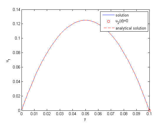
plot the numerical solution
plot(x,y)
xlabel('distance between plates')
ylabel('fluid velocity')
% the analytical solution to this problem is known, and we can plot it on
% top of the numerical solution
hold all
mu = 1;
d = 0.1
x = linspace(0,0.1);
Pdrop = -100; % this is DeltaP/Deltax
u = -(Pdrop)*d^2/2/mu*(x/d-(x/d).^2);
plot(x,u,'r--')
d =

    0.1000
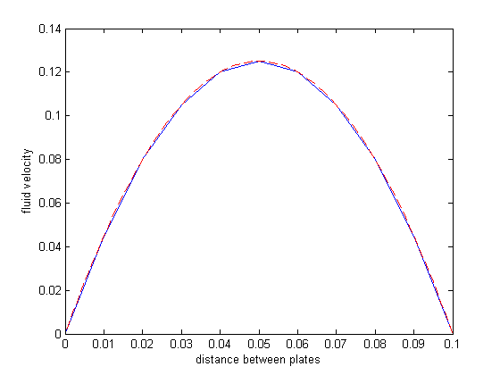
The two solutions agree. The advantages of this method over the shooting method (:postid:1036`) and builtin solver ( Post 878 ) are that you do not need to break the 2nd order ODE into a system of 1st order ODEs, and there is no "guessing" of the solution to get the solver started. Some disadvantages are the need to have a linear BVP in the form described at the beginning. If your BVP is nonlinear, you can't solve it with linear algebra! Another disadvantage is the amount of code we had to write. If you need to solve this kind of problem often, you probably would want to encapsulate the algorithm code into a reusable function.
'done'

% categories: ODEs
% tags: BVP

% post_id = 1193; %delete this line to force new post;
% permaLink = http://matlab.cheme.cmu.edu/2011/09/30/plane-poiseuelle-flow-solved-by-finite-difference/;
ans =

done
 between two stationary plates separated by distance
  and driven by a pressure drop
  , the governing equations on the velocity
  of the fluid are (assuming flow in the x-direction with the velocity varying only in the y-direction):
 and
and  , i.e. the no-slip condition at the edges of the plate.
 ,
,  and then
  . This leads to:

 and
and  .
. , and
, and  .
.