where its @ - I got two turntables and a microphone

| categories: basic matlab | View Comments

where its @ - I got two turntables and a microphone

where its @ - I got two turntables and a microphone

John Kitchin

Contents

Introduction

matlab allows you to define inline functions, known as function handles. These are helpful for making small functions that can be used with quad, fzero and the ode solvers without having to formally define function code blocks. One advantage of function handles is they can "see" all the variables in the script, so you don't have to copy the variables all over the place.

the syntax is: f = @(variables) expression-using-the-variables

then f(argument) is evaluated using the expression.

Here are some examples

make a function f(x) = 1/x^2

use dot operators to make the function vectorized. you should in general use the dot operators so your functions work with vectors, unless of course, your function uses linear algebra.

f = @(x) 1./x.^2;
f(2) % should equal 0.25
f([1 2 3]) % should equal [1 0.25 0.111]
ans =

    0.2500


ans =

    1.0000    0.2500    0.1111

you can have more than one variable, e.g. f(x,y)=x*y

f2 = @(x,y) x.*y;
f2(2,3) % should equal 6
f2([2 3],[3,4]) %should equal [6 12]
ans =

     6


ans =

     6    12

using function handles with quad

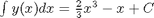
compute the integral of x^2 from 0 to 2

f3 = @(x) x.^3;
quad(f3,0,2) %the answer is 4
ans =

     4

using function handles with fzero

solve the equation x^2=9.5

myfunc = @(x) 9.5-x^2;
xguess = 3;
fzero(myfunc,xguess)
ans =

    3.0822

using function handles with ode45

solve y' = k*t over the time interval t=0 to 10, y(0)=3

k = 2.2;
myode = @(t,y) k*t;  % myode is a function handle
y0 = 3; tspan = [0 10];
[t,y] = ode45(myode,tspan,y0); % no @ on myode here because it is already
                               % a function handle
plot(t,y)
xlabel('Time')
ylabel('y')

% it is also possible to do coupled odes by defining anonymous functions,
% although not recommended! It's just harder to read than the functions.
%
%  solve
%
%  dX/dW = kp/Fao*(1-X)/(1+eps*X)*y
%  dy/dW = -alpha*(1+eps*X)/2/y
%  X(0) = 0, y(0)=1
%  we will let X = Y(1), y = Y(2)
eps = -0.15;
kp = 0.0266;
Fao = 1.08;
alpha = 0.0166;

myode2 = @(W,Y) [kp/Fao*(1-Y(1))./(1+eps*Y(1))*Y(2);
                 -alpha*(1+eps*Y(1))./(2*Y(2))];
[W,Y] = ode45(myode2,[0 60],[0 1]);
plot(W,Y(:,1),W,Y(:,2))
% even though you can do it, that doesn't mean it is easier to read! And
% shame on me for not labeling the plot axes.
'done'

% categories: Basic matlab
ans =

done

Read and Post Comments

Reading in delimited text files

| categories: basic matlab | View Comments

Reading in delimited text files

Reading in delimited text files

sometimes you will get data in a delimited text file format, .e.g. separated by commas or tabs. Matlab can read these in easily. Suppose we have a file containing this data ( download testdata.txt ):

1   3
3   4
5   6
4   8
% this is how you read it in.
A = textread('testdata.txt')

x = A(:,1);
y = A(:,2);

% you can do what ever you want with this data now. Plot it, integrate it,
% etc...

% categories: Basic matlab
% post_id = 722; %delete this line to force new post;
A =

     1     3
     3     4
     5     6
     4     8

Read and Post Comments

Read and Post Comments

polynomials in matlab

| categories: basic matlab | View Comments

polynomials

Contents

polynomials in matlab

polynomials can be represented as a vector of coefficients
4*x^3 + 3*x^2 -2*x + 10 = 0
can be represented as [4 3 -2 10]
ppar = [4 3 -2 10];

% we can evaluate the polynomial with the polyval command, e.g. to evaluate
% at x=3
polyval(ppar, 3)
ans =

   139

compare to

x=3;
4*x^3 + 3*x^2 -2*x + 10
% they are the same
ans =

   139

polynomial manipulations

matlab makes it easy to get the derivative and integral of a polynomial.

Consider:

$y = 2x^2 - 1$

ppar = [2 0 -1];

polynomial derivatives

$\frac{dy}{dx} = 4 x$

dpar = polyder(ppar)
% evaluate the derivative at x = 2
polyval(dpar,2)
dpar =

     4     0


ans =

     8

polynomial integrals

$\int y(x)dx = \frac{2}{3} x^3 - x + C$

We assume $C=0$.

ipar = polyint(ppar)
% note that the integration constant is assumed to be zero. If it is not
% zero, use POLYINT(P,K) where K is the constant of integration.
%
% Compute the integral of the polynomial from 2 to 4
polyval(ipar,4) - polyval(ipar,2)
% analytically:
2/3*(4^3 - 2^3) + (-4 - (-2))
ipar =

    0.6667         0   -1.0000         0


ans =

   35.3333


ans =

   35.3333

getting the roots of a polynomial

roots are the x-values that make the polynomial equal to zero.

roots(ppar)

% the analytical solutions are +- sqrt(1/2)

% note that imaginary roots exist, e.g. x^2 + 1 = 0 has two roots, +-i
ppar = [1 0 1]
roots(ppar)
ans =

    0.7071
   -0.7071


ppar =

     1     0     1


ans =

        0 + 1.0000i
        0 - 1.0000i

application in thermodynamics

we need to find the volume that solves the van der waal equation:

$$f(V) = V^3 - \frac{pnb + nRT}{p}V^2 + \frac{n^2a}{p}V - \frac{n^3ab}{p} = 0$$

where a and b are constants.

% numerical values of the constants
a = 3.49e4;
b = 1.45;
p = 679.7;
T = 683;
n = 1.136;
R = 10.73;

% The van der waal equation is a polynomial
%  V^3 - (p*n*b+n*R*T)/p*V^2 + n^2*a/p*V - n^3*a*b/p = 0

%use commas for clarity in separation of terms
ppar = [1, -(p*n*b+n*R*T)/p, n^2*a/p,  -n^3*a*b/p];
roots(ppar)

% note that only one root is real. In this case that means there is only
% one phase present.

% categories: Basic matlab
% tags: math, thermodynamics
ans =

   5.0943          
   4.4007 + 1.4350i
   4.4007 - 1.4350i

Read and Post Comments

Basic plotting tutorial

| categories: basic matlab, plotting | View Comments

Basic plotting tutorial

Basic plotting tutorial

Contents

it is a good idea to add these lines to the top of your m-files

close all  % close all figure windows that are open
clear all  % clear all the variables currently stored in memory
clc        % clear the commands in the command window

% Plotting functions in Matlab
% This m-file describes some very basic ways to plot functions in Matlab.

ezplot with functions described as strings

you can quickly plot a function of one variable with the ezplot command.

ezplot('x^3 - x^2 +x -1')
xlabel('x')
ylabel('f(x)')

plotting two functions with ezplot

if you try to plot another function, you will see the first function disappear. We have to tell Matlab what do with the hold command

figure
hold on
ezplot('x^3 - x^2 + x -1')
ezplot('-x^3 + x^2 - x + 1')
hold off

% Note that you cannot easily tell which graph is which because the two
% lines are the same color. Lets change the color and style of the first
% plot to be red and dashed, and add a legend so we can see which line is
% which. We do that by saving a reference to each figure in a variable so
% we can use the set function to modify each graph.

figure
hold on
h1 = ezplot('x^3 - x^2 + x -1');
h2 = ezplot('-x^3 + x^2 - x + 1');
hold off

set(h1,'color','r','linestyle','--')
legend('function 1','function2')

defining and plotting functions

strings are not always convenient to plot, especially if there are a lot of numbers in the equations, or if there are multiple variables. Let's plot the van der Waal's equation of state to show this.

$$f(V) = V^3 - \frac{pnb + nRT}{p}V^2 + \frac{n^2a}{p}V - \frac{n^3ab}{p} = 0$$

where a and b are constants. This equation cannot be plotted as a string like we did in the examples above. Instead, we need to define a function. Our goal is to find where this function is equal to zero. We can do that graphically.

% numerical values of the constants
a = 3.49e4;
b = 1.45;
p = 679.7;
T = 683;
n = 1.136;
R = 10.73;

% we define a function handle that is f(V)
f = @(V) V.^3 - (p*n*b+n*R*T)/p*V.^2 + n^2*a/p*V - n^3*a*b/p;

figure
ezplot(f)

%the large scale of the y-axis makes it difficult to see where the function
%is equal to zero, so we change the limits of each axis.
xlim([2 6])
ylim([-5 5])
xlabel('Volume')
ylabel('f(V)')
%it appears that f(V) = 0 around V=5
f(4.9)
f(5.1)
ans =

   -0.4486


ans =

    0.0145

we can add these two points to the figure with the plot command. Here we add them as red circles.

hold on
plot(4.9,f(4.9),'ro')
plot(5.1,f(5.1),'ro')
hold off

% The zero is definitely between V=4.9 and V = 5.1 because f changes sign
% between these two points.
%alternatively, we could tell ezplot to plot f from x=4 to x=6 like this
figure
ezplot(f,[4 6])
% categories: Basic Matlab, Plotting
% post_id = 625; %delete this line to force new post;
Read and Post Comments

« Previous Page -- Next Page »