Matlab in Chemical Engineering at CMU

Contents

curve fitting to get overlapping peak areas

John Kitchin

Today we examine an approach to fitting curves to overlapping peaks to deconvolute them so we can estimate the area under each curve. You will need to download gc-data-2.txt for this example. This file contains data from a gas chromatograph with two peaks that overlap. We want the area under each peak to estimate the gas composition. You will see how to read the text file in, parse it to get the data for plotting and analysis, and then how to fit it.

function main

read in the data file

The data file is all text, and we have to read it in, and find lines that match certain patterns to identify the regions that are data, then we read in the data lines.

clear all; close all

datafile = 'gc-data-2.txt';

fid = fopen(datafile);

first we get the number of data points, and read up to the data

i = 0;
while 1
    line = fgetl(fid);
    sm = strmatch('# of Points',line);
    if ~isempty(sm)
        regex = '# of Points(.*)';
        [match tokens] = regexp(line,regex,'match','tokens');
        npoints = str2num(tokens{1}{1});
    elseif strcmp(line,'R.Time	Intensity')
        break
    i = i + 1
    end
end

initialize the data vectors

t = zeros(1,npoints);
intensity = zeros(1,npoints);

now read in the data

for j=1:npoints
    line = fgetl(fid);
    [a] = textscan(line,'%f%d');
    t(j) = a{1};
    intensity(j) = a{2};
end

fclose(fid);

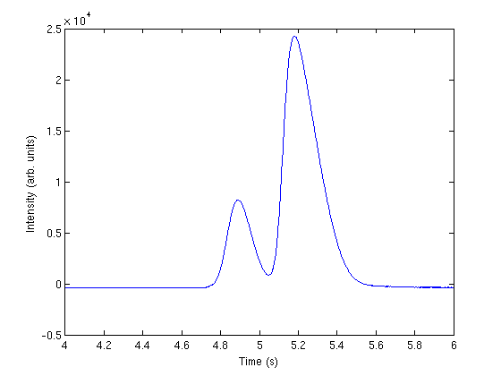
Plot the data

plot(t,intensity)
xlabel('Time (s)')
ylabel('Intensity (arb. units)')
xlim([4 6])

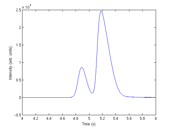
correct for non-zero baseline

intensity = intensity + 352;
plot(t,intensity)
xlabel('Time (s)')
ylabel('Intensity (arb. units)')
xlim([4 6])

a fitting function for one peak

The peaks are asymmetric, decaying gaussian functions.

    function f = asym_peak(pars,t)
        % from Anal. Chem. 1994, 66, 1294-1301
        a0 = pars(1);  % peak area
        a1 = pars(2);  % elution time
        a2 = pars(3);  % width of gaussian
        a3 = pars(4);  % exponential damping term
        f = a0/2/a3*exp(a2^2/2/a3^2 + (a1 - t)/a3)...
            .*(erf((t-a1)/(sqrt(2)*a2) - a2/sqrt(2)/a3) + 1);
    end

a fitting function for two peaks

to get two peaks, we simply add two peaks together.

    function f = two_peaks(pars, t)
        a10 = pars(1);  % peak area
        a11 = pars(2);  % elution time
        a12 = pars(3);  % width of gaussian
        a13 = pars(4);  % exponential damping term
        a20 = pars(5);  % peak area
        a21 = pars(6);  % elution time
        a22 = pars(7);  % width of gaussian
        a23 = pars(8);  % exponential damping term

        p1 = asym_peak([a10 a11 a12 a13],t);
        p2 = asym_peak([a20 a21 a22 a23],t);

        f = p1 + p2;
    end

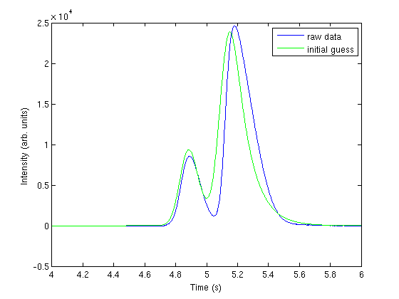
Plot fitting function with an initial guess for each parameter

the fit is not very good.

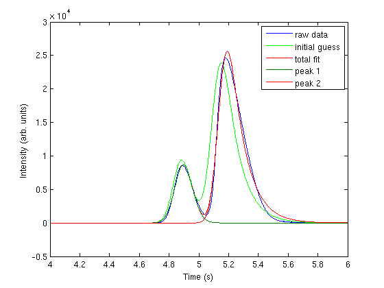
hold all;
parguess = [1500,4.85,0.05,0.05,5000,5.1,0.05,0.1];
plot (t,two_peaks(parguess,t),'g-')
legend 'raw data' 'initial guess'

nonlinear fitting

now we use nonlinear fitting to get the parameters that best fit our data, and plot the fit on the graph.

pars = nlinfit(t,intensity, @two_peaks, parguess)
plot(t,two_peaks(pars, t),'r-')
legend 'raw data' 'initial guess' 'total fit'

pars =

   1.0e+03 *

    1.3052    0.0049    0.0001    0.0000    5.3162    0.0051    0.0000    0.0001

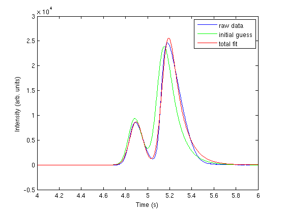
the fits are not perfect. The small peak is pretty good, but there is an unphysical tail on the larger peak, and a small mismatch at the peak. There is not much to do about that, it means the model peak we are using is not a good model for the peak. We will still integrate the areas though.

now extract out the two peaks and integrate the areas

pars1 = pars(1:4)
pars2 = pars(5:8)

peak1 = asym_peak(pars1, t);
peak2 = asym_peak(pars2, t);

plot(t,peak1)
plot(t,peak2)
legend 'raw data' 'initial guess' 'total fit' 'peak 1' 'peak 2';

area1 = trapz(t, peak1)
area2 = trapz(t, peak2)

pars1 =

   1.0e+03 *

    1.3052    0.0049    0.0001    0.0000


pars2 =

   1.0e+03 *

    5.3162    0.0051    0.0000    0.0001


area1 =

   1.3052e+03


area2 =

   5.3162e+03

Compute relative amounts

percent1 = area1/(area1 + area2)
percent2 = area2/(area1 + area2)

percent1 =

    0.1971


percent2 =

    0.8029

This sample was air, and the first peak is oxygen, and the second peak is nitrogen. we come pretty close to the actual composition of air, although it is low on the oxygen content. To do better, one would have to use a calibration curve.

end

% categories: data analysis

% post_id = 1994; %delete this line to force new post;
% permaLink = http://matlab.cheme.cmu.edu/2012/06/22/curve-fitting-to-get-overlapping-peak-areas/;

Published with MATLAB® 7.12