Matlab in Chemical Engineering at CMU

Contents

Constrained optimization

John Kitchin

adapted from http://en.wikipedia.org/wiki/Lagrange_multipliers.

function constrained_minimization

clear all; close all

Introduction

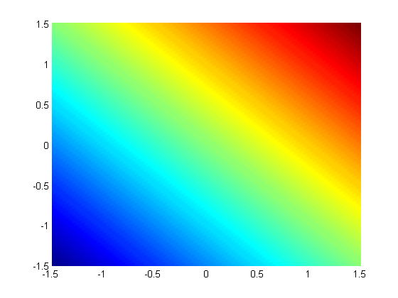
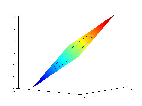
Suppose we seek to minimize the function subject to the constraint that . The function we seek to maximize is an unbounded plane, while the constraint is a unit circle. In Post 1602 we setup a Lagrange multiplier approach to solving this problem. Today, we use the builtin function fmincon in Matlab to solve the same problem.

We plot these two functions here.

x = linspace(-1.5,1.5);
[X,Y] = meshgrid(x,x);
figure; hold all
surf(X,Y,X+Y);
shading interp;

now plot the circle on the plane. First we define a circle in polar

coordinates, then convert those coordinates to x,y cartesian coordinates. then we plot f(x1,y1).

theta = linspace(0,2*pi);
[x1,y1] = pol2cart(theta,1);
plot3(x1,y1,x1+y1)
view(38,8) % adjust view so it is easy to see

Construct the function to optimize and the nonlinear constraint function

the original function, provided that the constraint is met!

    function f = func(X)
        x = X(1);
        y = X(2);
        f = x + y;
    end

    function [c,ceq] = nlconstraints(X)
        % function for the nonlinear constraints.
        % We have to define two outputs for fmincon: the nonlinear
        % inequality contraints, and the equality constraints.
        %
        % C(X) <= 0
        %
        % Ceq(X) = 0

        x = X(1);
        y = X(2);
        c = [];
        ceq = x^2 + y^2 - 1;
    end

Now we solve for the problem

fmincon takes a lot of options. We define all of them here, even though in this example we do not have any linear inequality or equality constraints, and we don't define bounds on the solution. It is necessary to put these empty placeholders in the fmincon call, however, so that it knows what the nonlinear constraints are.

A   =  [];
B   =  []; % the linear inequality constraints: A*X <= B
Aeq =  [];
Beq =  []; % the linear equality constraints: Aeq*X = B
LB  =  [];
UB  =  []; % LB <= X <= UB
X0  =  [1, 1]; % initial guess

[X,FVAL,EXITFLAG,OUTPUT,LAMBDA] = fmincon(@func,X0,A,B,Aeq,Beq,LB,UB,@nlconstraints)

OUTPUT.message
plot3(X(1),X(2),FVAL,'bo','markerfacecolor','b')

Warning: The default trust-region-reflective algorithm does not
solve problems with the constraints you have specified. FMINCON
will use the active-set algorithm instead. For information on
applicable algorithms, see Choosing the Algorithm in the
documentation. 

Local minimum possible. Constraints satisfied.

fmincon stopped because the predicted change in the objective function
is less than the default value of the function tolerance and constraints 
are satisfied to within the default value of the constraint tolerance.




X =

    0.7071    0.7071


FVAL =

    1.4142


EXITFLAG =

     5


OUTPUT = 

         iterations: 5
          funcCount: 15
       lssteplength: 1
           stepsize: 5.9440e-005
          algorithm: [1x44 char]
      firstorderopt: 7.9553e-006
    constrviolation: 2.3986e-011
            message: [1x776 char]


LAMBDA = 

         lower: [2x1 double]
         upper: [2x1 double]
         eqlin: [1x0 double]
      eqnonlin: 0.7071
       ineqlin: [1x0 double]
    ineqnonlin: [1x0 double]


ans =

Local minimum possible. Constraints satisfied.

fmincon stopped because the predicted change in the objective function
is less than the default value of the function tolerance and constraints 
are satisfied to within the default value of the constraint tolerance.

Stopping criteria details:

Optimization stopped because the predicted change in the objective function,
6.856786e-010, is less than options.TolFun = 1.000000e-006, and the maximum constraint
violation, 2.398637e-011, is less than options.TolCon = 1.000000e-006.

Optimization Metric                                                 Options
abs(steplength*directional derivative) =  6.86e-010        TolFun =  1e-006 (default)
max(constraint violation) =  2.40e-011                     TolCon =  1e-006 (default)

Note the warning about the algorithm change. Matlab automatically detected that it could not use the default algorithm because of the nonlinear constraints. Matlab also automatically selected a better algorithm for you.

There is a lot of output, that mostly tells us the function worked as expected. Note that the solution above is not a global minimum. There is another solution at the bottom of the circle. Let's try another initial guess.

X0 = [-1, -1];
[X,FVAL,EXITFLAG,OUTPUT,LAMBDA] = fmincon(@func,X0,A,B,Aeq,Beq,LB,UB,@nlconstraints)
plot3(X(1),X(2),FVAL,'ro','markerfacecolor','r')

Warning: The default trust-region-reflective algorithm does not
solve problems with the constraints you have specified. FMINCON
will use the active-set algorithm instead. For information on
applicable algorithms, see Choosing the Algorithm in the
documentation. 

Local minimum found that satisfies the constraints.

Optimization completed because the objective function is non-decreasing in 
feasible directions, to within the default value of the function tolerance,
and constraints are satisfied to within the default value of the constraint tolerance.




X =

   -0.7071   -0.7071


FVAL =

   -1.4142


EXITFLAG =

     1


OUTPUT = 

         iterations: 4
          funcCount: 15
       lssteplength: 1
           stepsize: 1.5019e-006
          algorithm: [1x44 char]
      firstorderopt: 1.0880e-008
    constrviolation: 2.2982e-012
            message: [1x787 char]


LAMBDA = 

         lower: [2x1 double]
         upper: [2x1 double]
         eqlin: [1x0 double]
      eqnonlin: 0.7071
       ineqlin: [1x0 double]
    ineqnonlin: [1x0 double]

This is the global minimum (by inspection).

Summary

the built in function fmincon is more flexible than what we did in Post 1602 since it includes inequality constraints. Of course, that flexibility comes at some cost, you have to know the expected syntax for each kind of constraint. But that is easy to find out with the Matlab documentation.

end

% categories: optimization

Published with MATLAB® 7.13