Plane Poiseuille flow - BVP solve by shooting method

In Post 878 learned how to use the BVP solver in Matlab to solve a boundary value problem. Another approach is to use the shooting method. The reason we can't use an initial value solver for a BVP is that there is not enough information at the initial value to start. In the shooting method, we take the function value at the initial point, and guess what the function derivatives are so that we can do an integration. If our guess was good, then the solution will go through the known second boundary point. If not, we guess again, until we get the answer we need. In this example we repeat the pressure driven flow example, but illustrate the shooting method.

In the pressure driven flow of a fluid with viscosity between two stationary plates separated by distance and driven by a pressure drop , the governing equations on the velocity of the fluid are (assuming flow in the x-direction with the velocity varying only in the y-direction):

Contents

with boundary conditions and , i.e. the no-slip condition at the edges of the plate.

we convert this second order BVP to a system of ODEs by letting , and then . This leads to:

with boundary conditions and .

for this problem we let the plate separation be d=0.1, the viscosity , and .

function main

clc; close all; clear all;

d = 0.1; % plate thickness

First guess

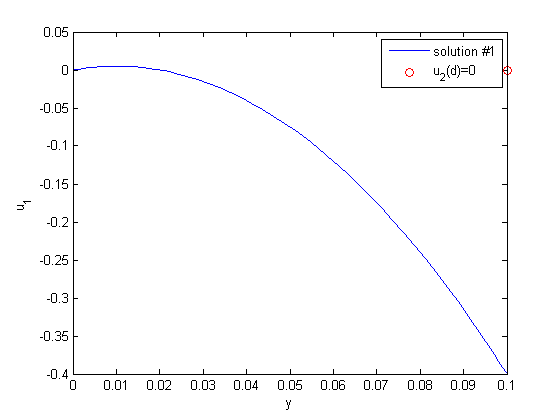
we need u_1(0) and u_2(0), but we only have u_1(0). We need to guess a value for u_2(0) and see if the solution goes through the u_2(d)=0 boundary value.

u1_0 = 0; % known
u2_0 = 1; % guessed

init = [u1_0 u2_0];
dspan = [0 d];
[y,U] = ode45(@odefun,dspan,init);
plot(y,U(:,1),[d],[0],'ro')
legend 'solution #1' 'u_2(d)=0'
xlabel('y')
ylabel('u_1')
% It appears we have undershot, so our initial slope was not large
% enough

second guess

u1_0 = 0; % known
u2_0 = 10; % guessed

init = [u1_0 u2_0];
dspan = [0 d];
[y,U] = ode45(@odefun,dspan,init);
plot(y,U(:,1),[d],[0],'ro')
legend 'solution #2' 'u_2(d)=0'
xlabel('y')
ylabel('u_1')
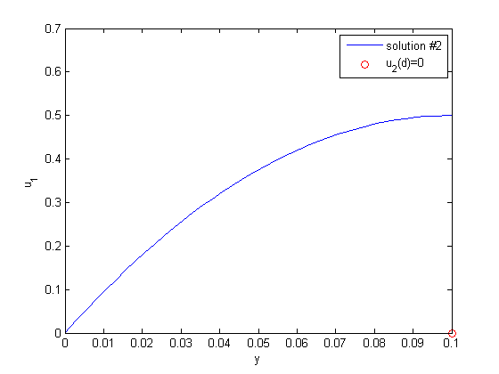
% Now we have overshot, the initial slope is too high. The right
% answer must be between 1 and 10 You could continue to iterate on
% this manually until the value of u_1(d) = 0. Instead, we use a
% solver to do that, now that we have a reasonable guess for u_2(0).

Using a solver

we have to make a function that is equal to zero when u_2(d) = 0.

u2_guess = 2;
u2_0_solved = fsolve(@myfunc,u2_guess)

Equation solved.

fsolve completed because the vector of function values is near zero
as measured by the default value of the function tolerance, and
the problem appears regular as measured by the gradient.




u2_0_solved =

    5.0000

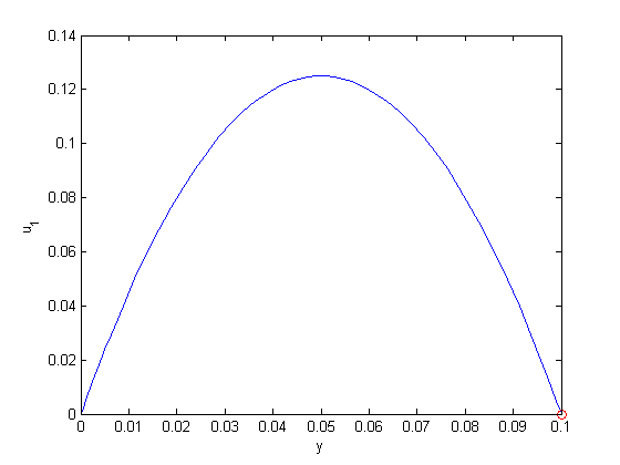
Plot final solution

init = [u1_0 u2_0_solved];
dspan = [0 d];
[y,U] = ode45(@odefun,dspan,init);

figure
plot(y,U(:,1),d,0,'ro')
xlabel('y')
ylabel('u_1')

Known analytical solution

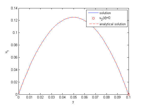
the analytical solution to this problem is known, and we can plot it on top of the numerical solution

mu = 1;
Pdrop = -100; % this is DeltaP/Deltax
u = -(Pdrop)*d^2/2/mu*(y/d-(y/d).^2);
hold all
plot(y,u,'r--')
legend 'solution' 'u_2(d)=0' 'analytical solution'

'done'

ans =

done

Finally, the solutions agree, and show that the velocity profile is parabolic, with a maximum in the middle of the two plates. You can also see that the velocity at each boundary is zero, as required by the boundary conditions

function dUdy = odefun(y,U)
% here we define our differential equations
u1 = U(1);
u2 = U(2);

mu = 1;
Pdrop = -100; % this is DeltaP/Deltax
du1dy = u2;
du2dy = 1/mu*Pdrop;
dUdy = [du1dy; du2dy];


function Z = myfunc(u2_guess)
% this function is zero when u_1(d) = 0.
u1_0 = 0; % known
u2_0 = u2_guess; % guessed
d = 0.1;

init = [u1_0 u2_0];
dspan = [0 d];
sol = ode45(@odefun,dspan,init);

u = deval(sol,d); % u = [u_1(d) u_2(d)]
u1_d = u(1);
Z = u1_d;

% categories: ODEs
% tags: math, fluids, bvp


% post_id = 1036; %delete this line to force new post;

Published with MATLAB® 7.12