Matlab in Chemical Engineering at CMU

Contents

Nonlinear curve fitting with parameter confidence intervals

John Kitchin

clear all; close all; clc

raw data to fit

x = [0.5 0.387 0.24 0.136 0.04 0.011];
y = [1.255 1.25 1.189 1.124 0.783 0.402];

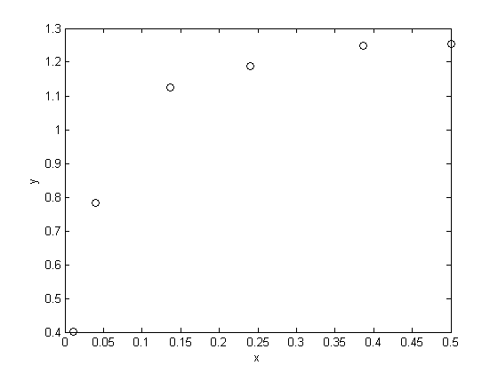
plot the data

you should usually plot your data to get a feel for how it looks.

plot(x,y,'ko')
xlabel('x')
ylabel('y')

nonlinear fitting

fit this nonlinear model y = Ax/(B+x) to the data. I use a function handle here, but I think it is cleaner and easier to read with a subfunction. here pars(1) = A, and pars(2) = B

f = @(pars,x) pars(1)*x./(pars(2)+x);

parguess = [ 1.3 0.03]; % nonlinear fits need initial guesses
[pars, resid, J] = nlinfit(x,y,f,parguess)

pars =

    1.3275    0.0265


resid =

   -0.0058    0.0074   -0.0067    0.0127   -0.0160    0.0122


J =

    0.9497   -2.3949
    0.9360   -3.0053
    0.9007   -4.4873
    0.8371   -6.8404
    0.6019  -12.0216
    0.2936  -10.4056

get the confidence interval for each parameter

the nlparci command estimates confidence intervals. The first row of the output is parameter 1, second row parameter 2, ...

alpha = 0.05; % this is for 95% confidence intervals
pars_ci = nlparci(pars,resid,'jacobian',J,'alpha',alpha)
sprintf('A is in the range of [%1.2f %1.2f] at the 95%% confidence level',pars_ci(1,:))
sprintf('B is in the range of [%1.2f %1.2f] at the 95%% confidence level',pars_ci(2,:))

pars_ci =

    1.3005    1.3545
    0.0236    0.0293


ans =

A is in the range of [1.30 1.35] at the 95% confidence level


ans =

B is in the range of [0.02 0.03] at the 95% confidence level

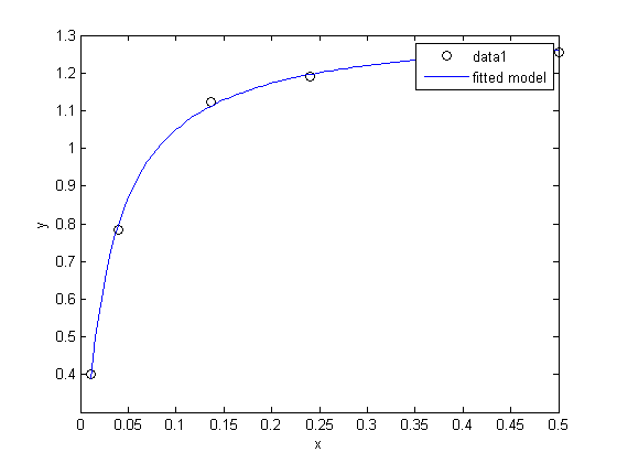
hold all
xfit = linspace(0.5, 0.011);
plot(xfit,f(pars,xfit),'DisplayName','fitted model')
legend show

summary

The fit looks reasonable, and the confidence intervals are "tight" and do not include zero, suggesting the parameters are significant.

% categories: data analysis

Published with MATLAB® 7.12