Matlab in Chemical Engineering at CMU

Solving Bessel's Equation numerically

August 08, 2011 at 01:53 PM | categories: odes | View Comments

Solving Bessel's Equation numerically

Reference Ch 5.5 Kreysig, Advanced Engineering Mathematics, 9th ed.

Bessel's equation $x^2 y'' + x y' + (x^2 - \nu^2)y=0$ comes up often in engineering problems such as heat transfer. The solutions to this equation are the Bessel functions. To solve this equation numerically, we must convert it to a system of first order ODEs. This can be done by letting $z = y'$ and $z' = y''$ and performing the change of variables:

$$ y' = z$$

$z' = \frac{1}{x^2}(-x z - (x^2 - \nu^2) y$

if we take the case where $\nu = 0$ , the solution is known to be the Bessel function $J_0(x)$ , which is represented in Matlab as besselj(0,x). The initial conditions for this problem are: $y(0) = 1$ and $y'(0)=0$ .

function bessel_ode

clear all; close all; clc;
% define the initial conditions
y0 = 1;
z0 = 0;
Y0 = [y0 z0];

There is a problem with our system of ODEs at x=0. Because of the $1/x^2$ term, the ODEs are not defined at x=0.

fbessel(0,Y0)

ans =

     0
   NaN

if we start very close to zero instead, we avoid the problem

fbessel(1e-15,Y0)

ans =

     0
    -1

xspan = [1e-15 10];
[x,Y] = ode45(@fbessel, xspan, Y0);

figure
hold on
plot(x,Y(:,1),'b-');
plot(x,besselj(0,x),'r--')
legend 'Numerical solution' 'analytical J_0(x)'

You can see the numerical and analytical solutions overlap, indicating they are the same.

'done'

ans =

done

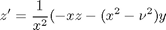
function dYdx = fbessel(x,Y)
% definition of the Bessel equation as a system of first order ODEs
nu = 0;

y = Y(1);
z = Y(2);

dydx = z;
dzdx = 1/x^2*(-x*z - (x^2 - nu^2)*y);

dYdx = [dydx; dzdx];

% categories: ODEs
% tags: math
% post_id = 763; %delete this line to force new post;