Contents

Estimating the boiling point of water

John Kitchin

I got distracted looking for Shomate parameters for ethane today, and came across this website on predicting the boiling point of water using the Shomate equations. The basic idea is to find the temperature where the Gibbs energy of water as a vapor is equal to the Gibbs energy of the liquid.

clear all; close all

Liquid water

http://webbook.nist.gov/cgi/cbook.cgi?ID=C7732185&Units=SI&Mask=2#Thermo-Condensed valid over 298-500

Hf_liq = -285.830; % kJ/mol
S_liq = 0.06995;   % kJ/mol/K
shomateL = [-203.6060
            1523.290
           -3196.413
            2474.455
               3.855326
            -256.5478
            -488.7163
            -285.8304];

Gas phase water

http://webbook.nist.gov/cgi/cbook.cgi?ID=C7732185&Units=SI&Mask=1&Type=JANAFG&Table=on#JANAFG

Interestingly, these parameters are listed as valid only above 500K. That means we have to extrapolate the values down to 298K. That is risky for polynomial models, as they can deviate substantially outside the region they were fitted to.

Hf_gas = -241.826; % kJ/mol
S_gas = 0.188835;  % kJ/mol/K

shomateG = [30.09200
             6.832514
             6.793435
            -2.534480
             0.082139
          -250.8810
           223.3967
          -241.8264];

Compute G over a range of temperatures.

T = linspace(0,200)' + 273.15; % temperature range from 0 to 200 degC

t = T/1000;

% normalize sTT by 1/1000  so entropies are in kJ/mol/K
sTT = [log(t) t t.^2/2 t.^3/3 -1./(2*t.^2) 0*t.^0 t.^0 0*t.^0]/1000;
hTT = [t t.^2/2 t.^3/3 t.^4/4 -1./t 1*t.^0 0*t.^0 -1*t.^0];

Gliq = Hf_liq + hTT*shomateL - T.*(sTT*shomateL);
Ggas = Hf_gas + hTT*shomateG - T.*(sTT*shomateG);

Interpolate the difference between the two vectors to find the boiling point

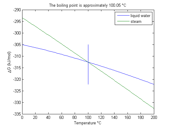
The boiling point is where Gliq = Ggas, so we solve Gliq(T)-Ggas(T)=0 to find the point where the two free energies are equal.

f = @(t) interp1(T,Gliq-Ggas,t);
bp = fzero(f,373)

bp =

  373.2045

Plot the two free energies

You can see the intersection occurs at approximately 100 degC.

plot(T-273.15,Gliq,T-273.15,Ggas)
line([bp bp]-273.15,[min(Gliq) max(Gliq)])
legend('liquid water','steam')
xlabel('Temperature \circC')
ylabel('\DeltaG (kJ/mol)')
title(sprintf('The boiling point is approximately %1.2f \\circC', bp-273.15))

Summary

The answer we get us 0.05 K too high, which is not bad considering we estimated it using parameters that were fitted to thermodynamic data and that had finite precision and extrapolated the steam properties below the region the parameters were stated to be valid for.

% tags: thermodynamics

Published with MATLAB® 7.13

Gibbs energy minimization and the NIST webbook

John Kitchin

Contents

In Post 1536 we used the NIST webbook to compute a temperature dependent Gibbs energy of reaction, and then used a reaction extent variable to compute the equilibrium concentrations of each species for the water gas shift reaction.

Today, we look at the direct minimization of the Gibbs free energy of the species, with no assumptions about stoichiometry of reactions. We only apply the constraint of conservation of atoms. We use the NIST Webbook to provide the data for the Gibbs energy of each species.

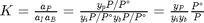
As a reminder we consider equilibrium between the species , , and , at 1000K, and 10 atm total pressure with an initial equimolar molar flow rate of and .

Links to data

H2

H2O

CO

CO2

function nist_wb_constrained_min

T = 1000; %K
R = 8.314e-3; % kJ/mol/K

P = 10; % atm, this is the total pressure in the reactor
Po = 1; % atm, this is the standard state pressure

We define species like this.

We are going to store all the data and calculations in vectors, so we need to assign each position in the vector to a species. Here are the definitions we use in this work.

1  CO
2  H2O
3  CO2
4  H2

species = {'CO' 'H2O' 'CO2' 'H2'};

Heats of formation at 298.15 K

Hf298 = [
    -110.53  % CO
    -241.826 % H2O
    -393.51  % CO2
       0.0]; % H2

Shomate parameters for each species

   A             B           C          D          E       F          G       H

WB = [25.56759  6.096130     4.054656  -2.671301  0.131021 -118.0089 227.3665   -110.5271  % CO
      30.09200  6.832514     6.793435  -2.534480  0.082139 -250.8810 223.3967   -241.8264    % H2O
      24.99735  55.18696   -33.69137    7.948387 -0.136638 -403.6075 228.2431   -393.5224   % CO2
      33.066178 -11.363417  11.432816  -2.772874 -0.158558 -9.980797 172.707974    0.0]; % H2

Shomate equations

t = T/1000;
T_H = [t; t^2/2; t^3/3; t^4/4; -1/t; 1; 0; -1];
T_S = [log(t); t; t^2/2; t^3/3; -1/(2*t^2); 0; 1; 0];

H = WB*T_H; % (H - H_298.15) kJ/mol
S = WB*T_S/1000; % absolute entropy kJ/mol/K

Gjo = Hf298 + H - T*S; % Gibbs energy of each component at 1000 K

Gibbs energy of mixture

this function assumes the ideal gas law for the activities

    function G = func(nj)
        Enj = sum(nj);
        G = sum(nj.*(Gjo'/R/T + log(nj/Enj*P/Po)));
    end

Elemental conservation constraints

We impose the constraint that all atoms are conserved from the initial conditions to the equilibrium distribution of species. These constraints are in the form of A_eq x = beq, where x is the vector of mole numbers. CO H2O CO2 H2

Aeq = [ 1    0    1    0   % C balance
        1    1    2    0   % O balance
        0    2    0    2]; % H balance

% equimolar feed of 1 mol H2O and 1 mol CO
beq = [1   % mol C fed
       2   % mol O fed
       2]; % mol H fed

Constraints on bounds

This simply ensures there are no negative mole numbers.

LB = [0 0 0];

Solve the minimization problem

x0 = [0.5 0.5 0.5 0.5]; % initial guesses

options = optimset('Algorithm','sqp');
x = fmincon(@func,x0,[],[],Aeq,beq,LB,[],[],options)

Local minimum found that satisfies the constraints.

Optimization completed because the objective function is non-decreasing in 
feasible directions, to within the default value of the function tolerance,
and constraints are satisfied to within the default value of the constraint tolerance.




x =

    0.4549    0.4549    0.5451    0.5451

Compute mole fractions and partial pressures

The pressures here are in good agreement with the pressures found in Post 1536 . The minor disagreement (in the third or fourth decimal place) is likely due to convergence tolerances in the different algorithms used.

yj = x/sum(x);
Pj = yj*P;

for i=1:numel(x)
    fprintf('%5d%10s%15.4f atm\n',i, species{i}, Pj(i))
end

    1        CO         2.2745 atm
    2       H2O         2.2745 atm
    3       CO2         2.7255 atm
    4        H2         2.7255 atm

Computing equilibrium constants

We can compute the equilibrium constant for the reaction . Compared to the value of K = 1.44 we found at the end of Post 1536 , the agreement is excellent. Note, that to define an equilibrium constant it is necessary to specify a reaction, even though it is not necessary to even consider a reaction to obtain the equilibrium distribution of species!

nuj = [-1 -1 1 1]; % stoichiometric coefficients of the reaction
K = prod(yj.^nuj)

K =

    1.4359

end

% categories: optimization
% tags: Thermodynamics, reaction engineering

Published with MATLAB® 7.12

Finding equilibrium composition by direct minimization of Gibbs free energy on mole numbers

John Kitchin

Adapted from problem 4.5 in Cutlip and Shacham

Contents

Problem setup

Ethane and steam are fed to a steam cracker at a total pressure of 1 atm and at 1000K at a ratio of 4 mol H2O to 1 mol ethane. Estimate the equilibrium distribution of products (CH4, C2H4, C2H2, CO2, CO, O2, H2, H2O, and C2H6).

Solution method: We will construct a Gibbs energy function for the mixture, and obtain the equilibrium composition by minimization of the function subject to elemental mass balance constraints.

function main

R = 0.00198588; % kcal/mol/K
T = 1000; % K

% we store the species names in a cell array since they have different
% lengths (i.e. different number of characters in names).
species = {'CH4' 'C2H4' 'C2H2' 'CO2' 'CO' 'O2' 'H2' 'H2O' 'C2H6'};

%
% $G_^\circ for each species. These are the heats of formation for each
% species.
Gjo = [4.61 28.249 40.604 -94.61 -47.942 0 0 -46.03 26.13]; % kcal/mol

The Gibbs energy of a mixture

We start with . Recalling that we define 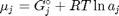, and in the ideal gas limit, , and that . Since in this problem, P = 1 atm, this leads to the function .

    function G = func(nj)
        Enj = sum(nj);
        G = sum(nj.*(Gjo/R/T + log(nj/Enj)));
    end

Linear equality constraints for atomic mass conservation

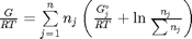The total number of each type of atom must be the same as what entered the reactor. These form equality constraints on the equilibrium composition. We express these constraints as: where is a vector of the moles of each species present in the mixture. CH4 C2H4 C2H2 CO2 CO O2 H2 H2O C2H6

Aeq = [0   0    0    2   1  2  0  1   0       % oxygen balance
       4   4    2    0   0  0  2  2   6       % hydrogen balance
       1   2    2    1   1  0  0  0   2];     % carbon balance

% the incoming feed was 4 mol H2O and 1 mol ethane
beq = [4    % moles of oxygen atoms coming in
       14   % moles of hydrogen atoms coming in
       2];  % moles of carbon atoms coming in

Bounds on mole numbers

No mole number can be negative, so we define a lower bound of zero for each mole number. In principle there are upper bounds too, but it is unecessary to define them here.

LB = [0 0 0 0 0 0 0 0 0]; % no mole numbers less than zero

initial guess for the solver

these are the guesses suggested in the book.

x0 = [1e-3 1e-3 1e-3 0.993 1 1e-4 5.992 1 1e-3]; % initial guess

Setup minimization

fmincon does not solve this problem with the default solver, and warns you to pick another one, either 'interior-point' or 'sqp'. Both work for this problem.

options = optimset('Algorithm','sqp');
[x fval] = fmincon(@func,x0,[],[],Aeq,beq,LB,[],[],options);

for i=1:numel(x)
    fprintf('%5d%10s%10.3g\n',i,species{i},x(i))
end

Local minimum possible. Constraints satisfied.

fmincon stopped because the size of the current step is less than
the default value of the step size tolerance and constraints are 
satisfied to within the default value of the constraint tolerance.



    1       CH4    0.0664
    2      C2H4 8.88e-008
    3      C2H2 2.76e-021
    4       CO2     0.545
    5        CO      1.39
    6        O2 4.56e-021
    7        H2      5.35
    8       H2O      1.52
    9      C2H6  1.6e-007

Verify the equality constraints were met

you can see here the constraints were met.

Aeq*x'
beq

ans =

     4
    14
     2


beq =

     4
    14
     2

Results

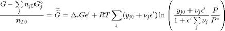
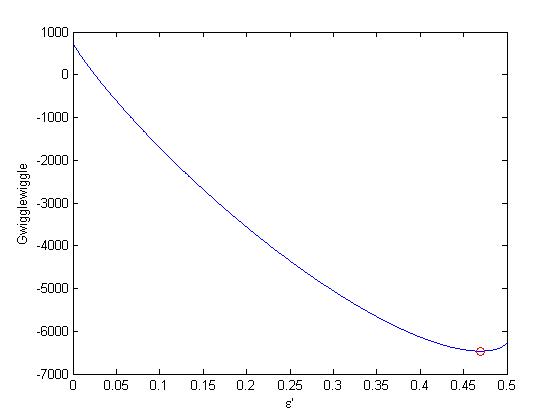
Interestingly there is a distribution of products! That is interesting because only steam and ethane enter the reactor, but a small fraction of methane is formed! The main product is hydrogen. The stoichiometry of steam reforming is ideally . Even though nearly all the ethane is consumed, we don't get the full yield of hydrogen. It appears that another equilibrium, one between CO, CO2, H2O and H2, may be limiting that, since the rest of the hydrogen is largely in the water. It is also of great importance that we have not said anything about reactions, i.e. how these products were formed. This is in stark contrast to Post 1589 where stoichiometric coefficients were necessary to perform the minimization.

Water gas shift equilibrium

The water gas shift reaction is: . We can compute the Gibbs free energy of the reaction from the heats of formation of each species. Assuming these are the formation energies at 1000K, this is the reaction free energy at 1000K.

G_wgs = Gjo(4) + Gjo(7) - Gjo(5) - Gjo(8)

G_wgs =

   -0.6380

WGS equilibrium constant at 1000K

exp(-G_wgs/R/T)

ans =

    1.3789

Equilibrium constant based on mole numbers

One normally uses activities to define the equilibrium constant. Since there are the same number of moles on each side of the reaction all factors that convert mole numbers to activity, concentration or pressure cancel, so we simply consider the ratio of mole numbers here.

x(4)*x(7)/(x(5)*x(8))

ans =

    1.3789

Clearly, there is an equilibrium between these species that prevents the complete reaction of steam reforming.

Summary

This is an appealing way to minimize the Gibbs energy of a mixture. No assumptions about reactions are necessary, and the constraints are easy to identify. The Gibbs energy function is especially easy to code.

end

% categories: optimization
% tags: Thermodynamics, reaction engineering
% post_id = 1630; %delete this line to force new post;
% permaLink = http://matlab.cheme.cmu.edu/2011/12/25/finding-equilibrium-composition-by-direct-minimization-of-gibbs-free-energy-on-mole-numbers/;

Published with MATLAB® 7.13

The Gibbs free energy of a reacting mixture and the equilibrium composition

John Kitchin

Adapted from Chapter 3 in Rawlings and Ekerdt.

Contents

Introduction

In this post we derive the equations needed to find the equilibrium composition of a reacting mixture. We use the method of direct minimization of the Gibbs free energy of the reacting mixture.

The Gibbs free energy of a mixture is defined as where is the chemical potential of species , and it is temperature and pressure dependent, and is the number of moles of species .

We define the chemical potential as , where is the Gibbs energy in a standard state, and is the activity of species if the pressure and temperature are not at standard state conditions.

If a reaction is occurring, then the number of moles of each species are related to each other through the reaction extent and stoichiometric coefficients: . Note that the reaction extent has units of moles.

Combining these three equations and expanding the terms leads to:

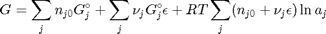
The first term is simply the initial Gibbs free energy that is present before any reaction begins, and it is a constant. It is difficult to evaluate, so we will move it to the left side of the equation in the next step, because it does not matter what its value is since it is a constant. The second term is related to the Gibbs free energy of reaction: . With these observations we rewrite the equation as:

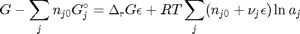
Now, we have an equation that allows us to compute the change in Gibbs free energy as a function of the reaction extent, initial number of moles of each species, and the activities of each species. This difference in Gibbs free energy has no natural scale, and depends on the size of the system, i.e. on . It is desirable to avoid this, so we now rescale the equation by the total initial moles present, and define a new variable , which is dimensionless. This leads to:

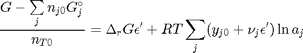
where is the initial mole fraction of species present. The mole fractions are intensive properties that do not depend on the system size. Finally, we need to address . For an ideal gas, we know that , where the numerator is the partial pressure of species computed from the mole fraction of species times the total pressure. To get the mole fraction we note:

This finally leads us to an equation that we can evaluate as a function of reaction extent:

we use a double tilde notation to distinguish this quantity from the quantity derived by Rawlings and Ekerdt which is further normalized by a factor of . This additional scaling makes the quantities dimensionless, and makes the quantity have a magnitude of order unity, but otherwise has no effect on the shape of the graph.

Finally, if we know the initial mole fractions, the initial total pressure, the Gibbs energy of reaction, and the stoichiometric coefficients, we can plot the scaled reacting mixture energy as a function of reaction extent. At equilibrium, this energy will be a minimum. We consider the example in Rawlings and Ekerdt where isobutane (I) reacts with 1-butene (B) to form 2,2,3-trimethylpentane (P). The reaction occurs at a total pressure of 2.5 atm at 400K, with equal molar amounts of I and B. The standard Gibbs free energy of reaction at 400K is -3.72 kcal/mol. Compute the equilibrium composition.

function main

clear all; close all

u = cmu.units;
R = 8.314*u.J/u.mol/u.K;
P = 2.5*u.atm;
Po = 1*u.atm; % standard state pressure
T = 400*u.K;

Grxn = -3.72*u.kcal/u.mol; %reaction free energy at 400K
yi0 = 0.5; yb0 = 0.5; yp0 = 0.0; % initial mole fractions

yj0 = [yi0 yb0 yp0];
nu_j = [-1 -1 1]; % stoichiometric coefficients

Define a function for

We will call this difference Gwigglewiggle.

    function diffG = Gfunc(extentp)
        diffG = Grxn*extentp;

        sum_nu_j = sum(nu_j);
        for i = 1:length(yj0)
            x1 = yj0(i) + nu_j(i)*extentp;
            x2 = x1./(1+extentp*sum_nu_j);
            diffG = diffG + R*T*x1.*log(x2*P/Po);
        end
    end

Plot function

There are bounds on how large can be. Recall that , and that . Thus, , and the maximum value that can have is therefore where . When there are multiple species, you need the smallest to avoid getting negative mole numbers.

epsilonp_max = min(-yj0(yj0>0)./nu_j(yj0>0))
epsilonp = linspace(0,epsilonp_max,1000);
plot(epsilonp,Gfunc(epsilonp))
xlabel('\epsilon''')
ylabel('Gwigglewiggle')

epsilonp_max =

    0.5000

Find extent that minimizes Gwigglewiggle

fminbnd is not defined for the units class, so we wrap the function in a function handle that makes it output a double. Alternatively, we could make the function fully dimensionless. We save that for a later post.

f = @(x) double(Gfunc(x))
epsilonp_eq = fminbnd(f,0,epsilonp_max)

hold on
plot(epsilonp_eq,Gfunc(epsilonp_eq),'ro')

f = 

    @(x)double(Gfunc(x))


epsilonp_eq =

    0.4696

Compute equilibrium mole fractions

yi = (yi0 + nu_j(1)*epsilonp_eq)/(1 + epsilonp_eq*sum(nu_j))
yb = (yb0 + nu_j(2)*epsilonp_eq)/(1 + epsilonp_eq*sum(nu_j))
yp = (yp0 + nu_j(3)*epsilonp_eq)/(1 + epsilonp_eq*sum(nu_j))

yi =

    0.0572


yb =

    0.0572


yp =

    0.8855

alternative way to compute mole fractions

y_j = (yj0 + nu_j*epsilonp_eq)/(1 + epsilonp_eq*sum(nu_j))

y_j =

    0.0572    0.0572    0.8855

Check for consistency with the equilibrium constant

K = exp(-Grxn/R/T)

K =

  108.1300

.

yp/(yi*yb)*Po/P

ans =

  108.0702

an alternative form of the equilibrium constant

We can express the equilibrium constant like this :$K = \prod\limits_j a_j^{\nu_j}$, and compute it with a single command.

prod((y_j*P/Po).^nu_j)

ans =

  108.0702

These results are very close, and only disagree because of the default tolerance used in identifying the minimum of our function. you could tighten the tolerances by setting options to the fminbnd function.

Summary

In this post we derived an equation for the Gibbs free energy of a reacting mixture and used it to find the equilibrium composition. In future posts we will examine some alternate forms of the equations that may be more useful in some circumstances.

end

% categories: optimization
% tags: thermodynamics, reaction engineering

Published with MATLAB® 7.13

Contents

Interacting with graphs with context menus

John Kitchin

In Post 1489 we saw how to interact with a contour plot using mouse clicks. That is helpful, but limited to a small number of click types, e.g. left or right clicks, double clicks, etc... And it is not entirely intuitive which one to use if you don't know in advance. In Post 1513 , we increased the functionality by adding key presses to display different pieces of information. While that significantly increases what is possible, it is also difficult to remember what keys to press when there are a lot of them!

Today we examine how to make a context menu that you access by right-clicking on the graph. After you select a menu option, some code is run to do something helpful. We will examine an enthalpy-pressure diagram for steam, and set up functions so you can select one a few thermodynamic functions to display the relevant thermodynamic property under the mouse cursor.

See the video.

function main

The XSteam module makes it pretty easy to generate figures of the steam tables. Here we make the enthalpy-pressure graph.

clear all; close all
P = logspace(-2,3,500); %bar

temps = [1 50 100 150 200 300 400 500 600 700 800]; % degC
figure; hold all
for Ti=temps
    Hh = @(p) XSteam('h_PT',p,Ti);
    H = arrayfun(Hh,P);
    plot(H,P,'k-')
    % add a text label to each isotherm of the temperature
    text(H(end),P(end),sprintf(' %d ^{\\circ}C',Ti),'rotation',90);
end

% add the saturated liquid line
hsat_l = arrayfun(@(p) XSteam('hL_p',p),P);
plot(hsat_l,P)

% add the saturated vapor line
hsat_v = arrayfun(@(p) XSteam('hV_p',p),P);
plot(hsat_v,P)

xlabel('Enthalpy (kJ/kg)')
ylabel('Pressure (bar)')
set(gca,'YScale','log') % this is the traditional view
% adjust axes position so the temperature labels aren't cutoff.
set(gca,'Position',[0.13 0.11 0.775 0.7])

Now we add a textbox to the graph where we will eventually print the thermodynamic properties. We also put a tooltip on the box, which will provide some help if you hold your mouse over it long enough.

textbox_handle = uicontrol('Style','text',...
    'String','Hover mouse here for help',...
     'Position', [0 0 200 25],...
     'TooltipString','Right-click to get a context menu to select a thermodynamic property under the mouse cursor.');

% we will create a simple cursor to show us what point the printed property
% corresponds too
cursor_handle = plot(0,0,'r+');

setup the context menu

hcmenu = uicontextmenu;

Define the context menu items

item1 = uimenu(hcmenu, 'Label', 'H', 'Callback', @hcb1);
item2 = uimenu(hcmenu, 'Label', 'S', 'Callback', @hcb2);
item3 = uimenu(hcmenu, 'Label', 'T', 'Callback', @hcb3);

Now we define the callback functions

    function hcb1(~,~)
        % called when H is selected from the menu
        current_point = get(gca,'Currentpoint');
        H = current_point(1,1);
        P = current_point(1,2);
        set(cursor_handle,'Xdata',H,'Ydata',P)

        % We read H directly from the graph
        str = sprintf('H   = %1.4g kJ/kg', H);
        set(textbox_handle, 'String',str,...
            'FontWeight','bold','FontSize',12)
    end

    function hcb2(~,~)
        % called when S is selected from the menu
        current_point = get(gca,'Currentpoint');
        H = current_point(1,1);
        P = current_point(1,2);
        set(cursor_handle,'Xdata',H,'Ydata',P)

        % To get S, we first need the temperature at the point
        % selected
        T = fzero(@(T) H - XSteam('h_PT',P,T),[1 800]);
        % then we compute the entropy from XSteam
        str = sprintf('S   = %1.4g kJ/kg/K',XSteam('s_PT',P,T));
        set(textbox_handle, 'String',str,...
            'FontWeight','bold','FontSize',12)
    end

    function hcb3(~,~)
        % called when T is selected from the menu
        current_point = get(gca,'Currentpoint');
        H = current_point(1,1);
        P = current_point(1,2);
        set(cursor_handle,'Xdata',H,'Ydata',P)

        % We have to compute the temperature that is consistent with
        % the H,P point selected
        T = fzero(@(T) H - XSteam('h_PT',P,T),[1 800]);
        str = sprintf('T   = %1.4g C',  T);
        set(textbox_handle, 'String',str,...
            'FontWeight','bold','FontSize',12)
    end

set the context menu on the current axes and lines

set(gca,'uicontextmenu',hcmenu)

hlines = findall(gca,'Type','line');
% Attach the context menu to each line
for line = 1:length(hlines)
    set(hlines(line),'uicontextmenu',hcmenu)
end

end

% categories: plotting
% tags: interactive, thermodynamics

Published with MATLAB® 7.13