Smooth transitions between discontinuous functions
October 30, 2011 at 05:12 PM | categories: miscellaneous, nonlinear algebra | View Comments
Contents
Smooth transitions between discontinuous functions
John Kitchin
In Post 1280 we used a correlation for the Fanning friction factor for turbulent flow in a pipe. For laminar flow (Re < 3000), there is another correlation that is commonly used:  . Unfortunately, the correlations for laminar flow and turbulent flow have different values at the transition that should occur at Re = 3000. This discontinuity can cause a lot of problems for numerical solvers that rely on derivatives.
Today we examine a strategy for smoothly joining these two functions.
function main
clear all; close all; clc
Friction factor correlations
    function f = fF_laminar(Re)
        f = 16./Re;
    end

    function f = fF_turbulent(Re)
        % Nikuradse correlation for turbulent flow
        function f = internalfunc(Re)
            f = fzero(@(f) 1/sqrt(f) - (4.0*log10(Re*sqrt(f))-0.4), 0.01);
        end
        % this makes the function act as if it were vectorized, so we can
        % get an array of friction factors
        f = arrayfun(@internalfunc,Re);
    end
Plot the correlations
Re1 = linspace(500,3000);
f1 = fF_laminar(Re1);

Re2 = linspace(3000,10000);
f2 = fF_turbulent(Re2);

figure(1)
plot(Re1,f1,Re2,f2)
xlabel('Re')
ylabel('f_F')
You can see the discontinuity at Re = 3000. What we need is a method to join these two functions smoothly. We can do that with a sigmoid function.
Sigmoid functions
A sigmoid function smoothly varies from 0 to 1 according to the equation: 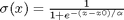 . The transition is centered on
 ![]() , and
, and  determines the width of the transition.
x = linspace(-4,4);
y = 1./(1+exp(-x/0.1));
figure(2)
plot(x,y)
xlabel('x'); ylabel('y'); title('\sigma(x)')
If we have two functions,  and
and  we want to smoothly join, we do it like this:
  . There is no formal justification for this form of joining, it is simply a mathematical convenience to get a numerically smooth function. Other functions besides the sigmoid function could also be used, as long as they smoothly transition from 0 to 1, or from 1 to zero.
Smoothly transitioning function to estimate friction factor
    function f = fanning_friction_factor(Re)
        % combined, continuous correlation for the fanning friction factor.
        % the alpha parameter is chosen to provide the desired smoothness.
        % The transition region is about +- 4*alpha. The value 450 was
        % selected to reasonably match the shape of the correlation
        % function provided by Morrison (see last section of this file)
        sigma =  1./(1+exp(-(Re - 3000)/450));
        f = (1-sigma).*fF_laminar(Re) + sigma.*fF_turbulent(Re);
    end

Re = linspace(500,10000);
f = fanning_friction_factor(Re);

figure(1); hold all
plot(Re,f)
xlabel('Re')
ylabel('f_F')
legend 'laminar' 'turbulent' 'smooth transition'
Exiting fzero: aborting search for an interval containing a sign change
    because complex function value encountered during search.
(Function value at -0.0028 is -5.2902-21.627i.)
Check function or try again with a different starting value.
You can see that away from the transition the combined function is practically equivalent to the original two functions. That is because away from the transition the sigmoid function is 0 or 1. Near Re = 3000 is a smooth transition from one curve to the other curve.
Morrison derived a single function for the friction factor correlation over all Re: 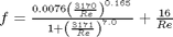 . Here we show the comparison with the approach used above. The friction factor differs slightly at high Re, becauase Morrison's is based on the Prandlt correlation, while the work here is based on the Nikuradse correlation. They are similar, but not the same.
h = plot(Re,16./Re + (0.0076*(3170./Re).^0.165)./(1 + (3170./Re).^7))

% Append an entry to the legend
[LEGH,OBJH,OUTH,OUTM] = legend;
% Add object with new handle and new legend string to legend
legend([OUTH;h],OUTM{:},'Morrison')
h =

  415.0735
Summary
The approach demonstrated here allows one to smoothly join two discontinuous functions that describe physics in different regimes, and that must transition over some range of data. It should be emphasized that the method has no physical basis, it simply allows one to create a mathematically smooth function, which could be necessary for some optimizers or solvers to work.
end % main

% categories: Miscellaneous, nonlinear algebra
% tags: Fluids
 , and the corresponding pressure drop is given by
  . In these equations,
  is the fluid density,
  is the fluid velocity,
  is the pipe diameter, and
  is the Fanning friction factor. The average fluid velocity is given by
  .
. , which is a linear equation, and for turbulent flow (
 ) we have the implicit equation
 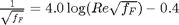 . Of course, we define
  where
where  is the viscosity of the fluid.
 and
and  where
where 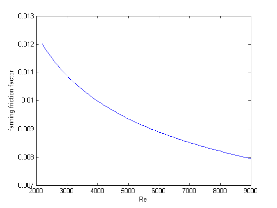
 that solves: $ \Delta p = \rho 2 f_F \frac{\Delta L v^2}{D}$. This is a nonlinear equation in
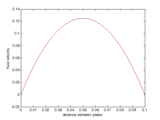
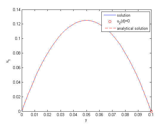
  between two stationary plates separated by distance
  and driven by a pressure drop
  , the governing equations on the velocity
  of the fluid are (assuming flow in the x-direction with the velocity varying only in the y-direction):
 and
and  , i.e. the no-slip condition at the edges of the plate.
 ,
,  and then
  . This leads to:

 and
and  .
. , and
, and  .
.
 between two stationary plates separated by distance
  and driven by a pressure drop
  , the governing equations on the velocity
  of the fluid are (assuming flow in the x-direction with the velocity varying only in the y-direction):
 and
and  , i.e. the no-slip condition at the edges of the plate.
 ,
,  and then
  . This leads to:

 and
and  .
. , and
, and  .
.