Contents
Error tolerance in numerical solutions to ODEs
Usually, the numerical solvers in Matlab work well with the standard settings. Sometimes they do not, and it is not always obvious they have not worked! Part of using a tool like Matlab is checking how well your solution really worked. We use an example of integrating an ODE that defines the van der Waal equation of an ideal gas here.
function vdw_tolerance
clc; clear all; close all
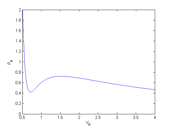
Analytical solution we are looking for
we plot the analytical solution to the van der waal equation in reduced form here.
Tr = 0.9;
Vr = linspace(0.34,4,1000);
Prfh = @(Vr) 8/3*Tr./(Vr - 1/3) - 3./(Vr.^2);
Pr = Prfh(Vr);
plot(Vr,Pr)
ylim([0 2])
xlabel('V_R')
ylabel('P_R')
Derive the ODE
we want an equation for dPdV, which we will integrate we use symbolic math to do the derivative for us.
syms Vrs Trs
Prs = 8/3*Tr./(Vrs - 1/3) - 3./(Vrs.^2) ;
diff(Prs,Vrs)
ans =
6/Vrs^3 - 12/(5*(Vrs - 1/3)^2)
Solve ODE with ode45
Vspan = [0.34 4];
Po = Prfh(Vspan(1));
[V,P] = ode45(@myode,Vspan,Po);
hold all
plot(V,P)
That is strange, the numerical solution does not agree with the analytical solution. Let's try a few more solvers:
[V,P] = ode15s(@myode,Vspan,Po);
plot(V,P)
[V,P] = ode113(@myode,Vspan,Po);
plot(V,P)
legend 'analytical' 'ode45' 'ode15s' 'ode113'
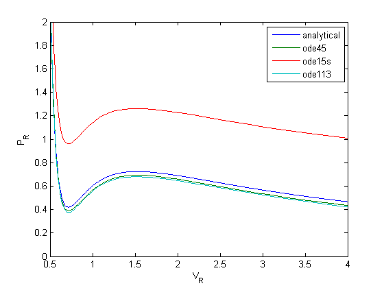
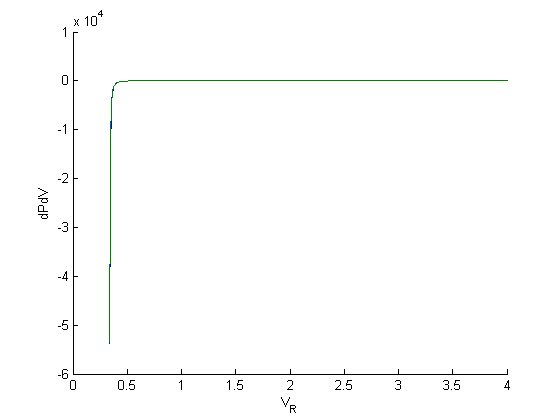
None of the solvers give good solutions! Let's take a look at the problem. First, look at the derivative values
figure; hold all
plot(Vr,myode(Vr,P))
plot(V,cmu.der.derc(V,P))
xlabel('V_R')
ylabel('dPdV')
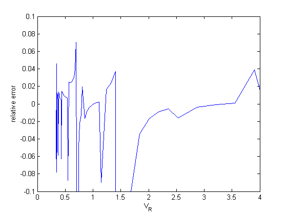
analysis of relative error
dPdV = cmu.der.derc(V,P);
error = (dPdV - myode(V,P))./dPdV;
figure
plot(V,error)
xlabel('V_R')
ylabel('relative error')
ylim([-0.1 0.1])
tighten the tolerances
We tighten the tolerances from 1e-3 (the default) to 1e-9
options = odeset('AbsTol',1e-9,'RelTol',1e-9);
[V,P] = ode45(@myode,[0.34,4], Prfh(0.34),options);
figure
hold all
plot(Vr,Pr)
plot(V,P,'r--')
ylim([0 2])
xlabel('V_R')
ylabel('P_R')
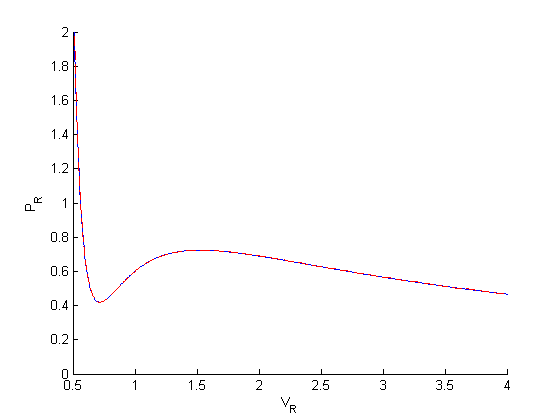
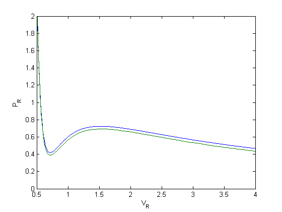
you can see much closer agreement with the analytical solution now.
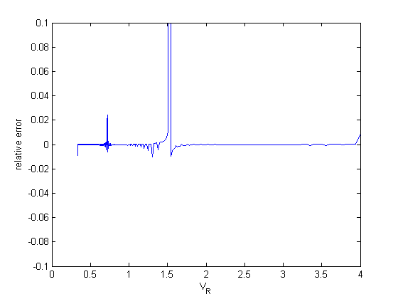
analysis of relative errors
Now, the errors are much smaller, with a few exceptions that don't have a big impact on the solution.
dPdV = cmu.der.derc(V,P);
error = (dPdV - myode(V,P))./dPdV;
figure
plot(V,error)
xlabel('V_R')
ylabel('relative error')
ylim([-0.1 0.1])
Summary
The problem here was the derivative value varied by four orders of magnitude over the integration range, so the default tolerances were insufficient to accurately estimate the numerical derivatives over that range. Tightening the tolerances helped resolve that problem. Another approach might be to split the integration up into different regions. For instance, if instead of starting at Vr = 0.34, which is very close to a sigularity in the van der waal equation at Vr = 1/3, if you start at Vr = 0.5, the solution integrates just fine with the standard tolerances.
'done'
ans =

done
function dPrdVr = myode(Vr,Pr)
dPrdVr = 6./Vr.^3 - 12./(5*(Vr - 1/3).^2);
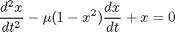
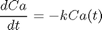
 is a constant. If we let
  http://en.wikipedia.org/wiki/Van_der_Pol_oscillator, then we arrive at this set of equations:
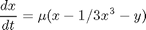

 .
.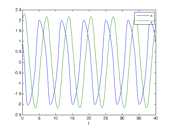
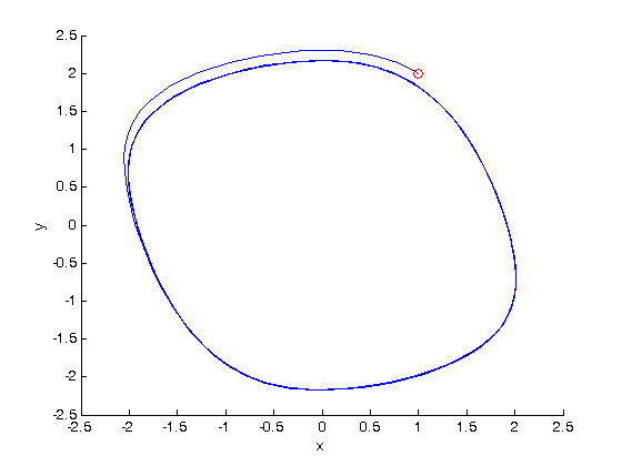
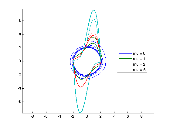
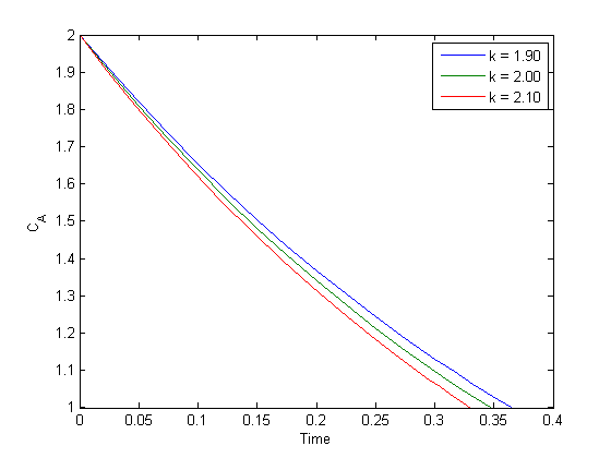
 is a parameter, and we want to solve the equation for a couple of values of
  , how long does it take to get
  , and how sensitive is the answer to small variations in