A novel way to numerically estimate the derivative of a function - complex-step derivative approximation

| categories: miscellaneous | View Comments

A novel way to numerically estimate the derivative of a function - complex-step derivative approximation

A novel way to numerically estimate the derivative of a function - complex-step derivative approximation

John Kitchin

Adapted from http://biomedicalcomputationreview.org/2/3/8.pdf and http://dl.acm.org/citation.cfm?id=838250.838251

This posts introduces a novel way to numerically estimate the derivative of a function that does not involve finite difference schemes. Finite difference schemes are approximations to derivatives that become more and more accurate as the step size goes to zero, except that as the step size approaches the limits of machine accuracy, new errors can appear in the approximated results. In the references above, a new way to compute the derivative is presented that does not rely on differences!

The new way is: $f'(x) = \rm{imag}(f(x + i\Delta x)/\Delta x)$ where the function $f$ is evaluated in imaginary space with a small $\Delta x$ in the complex plane. The derivative is miraculously equal to the imaginary part of the result in the limit of $\Delta x \rightarrow 0$!

Contents

Example 1

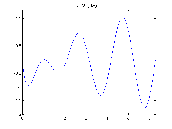
This example comes from the first link. The derivative must be evaluated using the chain rule. We compare a forward difference, central difference and complex-step derivative approximations.

f = @(x) sin(3*x)*log(x);
ezplot(f)

format long

at x = 0.7

x = 0.7;
h = 1e-7;

analytical derivative

dfdx_a = 3*cos(3*x)*log(x) + sin(3*x)/x
dfdx_a =

   1.773354106237345

finite difference

dfdx_fd = (f(x) - f(x-h))/h
dfdx_fd =

   1.773354270651062

central difference

dfdx_cd = (f(x+h)-f(x-h))/(2*h)
dfdx_cd =

   1.773354105227831

complex method

dfdx_I = imag(f(x+h*i)/h)
dfdx_I =

   1.773354106237384

compute errors

You can see the complex-step derivative approximation is several orders of magnitude more accurate than either of the finite difference methods.

dfdx_fd - dfdx_a
dfdx_cd - dfdx_a
dfdx_I - dfdx_a
ans =

    1.644137173073546e-007


ans =

   -1.009513361793779e-009


ans =

    3.952393967665557e-014

another example

Let's use this method to verify the fundamental Theorem of Calculus, i.e. to evaluate the derivative of an integral function. Let $f(x) = \int\limits_1^{x^2} tan(t^3)dt$
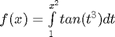
, and we now want to compute df/dx. Of course, this can be done analytically, but it is not trivial!

integrand = @(t) tan(t.^3);
f = @(z) quad(integrand, 0,z.^2);

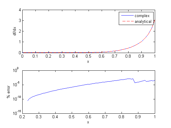
Lets evaluate the derivative over a range of x-values. The quad function is not vectorized for the limits, so we have to use arrayfun to map each x-value onto a vector of dfdx. The agreement here is very good, with the largest %%error being 0.0001%% near x=1. That interestingly does not get much better with smaller h.

x = linspace(0,1);
dfdx = imag(arrayfun(f,(x+i*h))/h);
dfdx_analytical = 2*x.*tan(x.^6);

subplot(2,1,1)
plot(x,dfdx,x,dfdx_analytical,'r--')
xlabel('x')
ylabel('df/dx')
legend('complex','analytical')

subplot(2,1,2)
semilogy(x,(dfdx-dfdx_analytical)./dfdx_analytical*100)
xlabel('x')
ylabel('% error')

don't get too complacent though!

Here is an example that fails to agree!

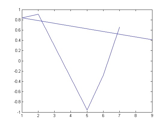
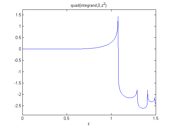
x = linspace(0,1.5);

dfdx = imag(arrayfun(f,(x+i*h))/h);
dfdx_analytical = 2*x.*tan(x.^6);

figure
plot(x,dfdx,x,dfdx_analytical,'r--')
legend('complex','analytical','location','best')

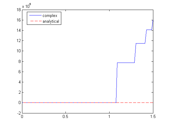
I guess the reason for the failure appears to be related to the singularity at x = 1.1. It is not clear why that causes the estimated derivative to blow up though, since it works everywhere else. It appears there is a step change at each singularity in the function.
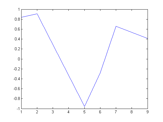
ezplot(f,[0,1.5])

Summary

Using this simple formula $f'(x) = imag(f(x + ih)/h)$ to approximate a derivative is one of the most interesting math facts I can't believe I didn't know before this post!

% categories: Miscellaneous
Read and Post Comments

Water gas shift equilibria via the NIST Webbook

| categories: miscellaneous, nonlinear algebra | View Comments

Water gas shift equilibria via the NIST Webbook

Water gas shift equilibria via the NIST Webbook

John Kitchin

The NIST webbook provides parameterized models of the enthalpy, entropy and heat capacity of many molecules. In this example, we will examine how to use these to compute the equilibrium constant for the water gas shift reaction $CO + H_2O \rightleftharpoons CO_2 + H_2$ in the temperature range of 500K to 1000K.

Parameters are provided for:

Contents

   Cp = heat capacity (J/mol*K)
   H° = standard enthalpy (kJ/mol)
   S° = standard entropy (J/mol*K)

with models in the form: $Cp^\circ = A + B*t + C*t^2 + D*t^3 +  E/t^2$

$H^\circ - H^\circ_{298.15}= A*t + B*t^2/2 +  C*t^3/3 + D*t^4/4 - E/t + F - H$

$S^\circ = A*ln(t) + B*t + C*t^2/2 + D*t^3/3 -  E/(2*t^2) + G$

where $t=T/1000$, and $T$ is the temperature in Kelvin. We can use this data to calculate equilibrium constants in the following manner. First, we have heats of formation at standard state for each compound; for elements, these are zero by definition, and for non-elements, they have values available from the NIST webbook. There are also values for the absolute entropy at standard state. Then, we have an expression for the change in enthalpy from standard state as defined above, as well as the absolute entropy. From these we can derive the reaction enthalpy, free energy and entropy at standard state, as well as at other temperatures.

We will examine the water gas shift enthalpy, free energy and equilibrium constant from 500K to 1000K, and finally compute the equilibrium composition of a gas feed containing 5 atm of CO and H2 at 1000K.

close all; clear all; clc;

T = linspace(500,1000); % degrees K
t = T/1000;

Setup equations for each species

First we enter in the parameters and compute the enthalpy and entropy for each species.

Hydrogen

link

% T = 298-1000K valid temperature range
A =  33.066178;
B = -11.363417;
C =  11.432816;
D = -2.772874;
E = -0.158558;
F = -9.980797;
G =  172.707974;
H =  0.0;

Hf_29815_H2 = 0.0; % kJ/mol
S_29815_H2 = 130.68; % J/mol/K

dH_H2 = A*t + B*t.^2/2 + C*t.^3/3 + D*t.^4/4 - E./t + F - H;
S_H2 = (A*log(t) + B*t + C*t.^2/2 + D*t.^3/3 - E./(2*t.^2) + G);

H2O

link Note these parameters limit the temperature range we can examine, as these parameters are not valid below 500K. There is another set of parameters for lower temperatures, but we do not consider them here.

% 500-1700 K valid temperature range
A =   30.09200;
B =   6.832514;
C =   6.793435;
D =  -2.534480;
E =   0.082139;
F =  -250.8810;
G =   223.3967;
H =  -241.8264;

Hf_29815_H2O = -241.83; %this is Hf.
S_29815_H2O = 188.84;

dH_H2O = A*t + B*t.^2/2 + C*t.^3/3 + D*t.^4/4 - E./t + F - H;
S_H2O = (A*log(t) + B*t + C*t.^2/2 + D*t.^3/3 - E./(2*t.^2) + G);

CO

link

% 298. - 1300K valid temperature range
A =   25.56759;
B =   6.096130;
C =   4.054656;
D =  -2.671301;
E =   0.131021;
F =  -118.0089;
G =   227.3665;
H = -110.5271;

Hf_29815_CO = -110.53; %this is Hf kJ/mol.
S_29815_CO = 197.66;

dH_CO = A*t + B*t.^2/2 + C*t.^3/3 + D*t.^4/4 - E./t + F - H;
S_CO = (A*log(t) + B*t + C*t.^2/2 + D*t.^3/3 - E./(2*t.^2) + G);

CO2

link

% 298. - 1200.K valid temperature range
A =   24.99735;
B =   55.18696;
C =  -33.69137;
D =   7.948387;
E =  -0.136638;
F =  -403.6075;
G =   228.2431;
H =  -393.5224;

Hf_29815_CO2 = -393.51; %this is Hf.
S_29815_CO2 = 213.79;

dH_CO2 = A*t + B*t.^2/2 + C*t.^3/3 + D*t.^4/4 - E./t + F - H;
S_CO2 = (A*log(t) + B*t + C*t.^2/2 + D*t.^3/3 - E./(2*t.^2) + G);

Standard state heat of reaction

We compute the enthalpy and free energy of reaction at 298.15 K for the following reaction $CO + H2O \rightleftharpoons H2 + CO2$.

Hrxn_29815 = Hf_29815_CO2 + Hf_29815_H2 - Hf_29815_CO - Hf_29815_H2O;
Srxn_29815 = S_29815_CO2 + S_29815_H2 - S_29815_CO - S_29815_H2O;
Grxn_29815 = Hrxn_29815 - 298.15*(Srxn_29815)/1000;

sprintf('deltaH = %1.2f',Hrxn_29815)
sprintf('deltaG = %1.2f',Grxn_29815)
ans =

deltaH = -41.15


ans =

deltaG = -28.62

Correcting $\Delta H$ and $\Delta G$

we have to correct for temperature change away from standard state. We only correct the enthalpy for this temperature change. The correction looks like this:

$$ \Delta H_{rxn}(T) = \Delta H_{rxn}(T_{ref}) + \sum_i \nu_i
(H_i(T)-H_i(T_{ref}))$$

Where $\nu_i$ are the stoichiometric coefficients of each species, with appropriate sign for reactants and products, and $(H_i(T)-H_i(T_{ref})$ 
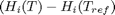
is precisely what is calculated for each species with the equations

Hrxn = Hrxn_29815 + dH_CO2 + dH_H2 - dH_CO - dH_H2O;

The entropy is on an absolute scale, so we directly calculate entropy at each temperature. Recall that H is in kJ/mol and S is in J/mol/K, so we divide S by 1000 to make the units match.

Grxn = Hrxn - T.*(S_CO2 + S_H2 - S_CO - S_H2O)/1000;

Plot how the $\Delta G$ varies with temperature

over this temperature range the reaction is exothermic, although near 1000K it is just barely exothermic. At higher temperatures we expect the reaction to become endothermic.

figure; hold all
plot(T,Grxn)
plot(T,Hrxn)
xlabel('Temperature (K)')
ylabel('(kJ/mol)')
legend('\Delta G_{rxn}', '\Delta H_{rxn}', 'location','best')

Equilibrium constant calculation

Note the equilibrium constant starts out high, i.e. strongly favoring the formation of products, but drops very quicky with increasing temperature.

R = 8.314e-3; %kJ/mol/K
K = exp(-Grxn/R./T);

figure
plot(T,K)
xlim([500 1000])
xlabel('Temperature (K)')
ylabel('Equilibrium constant')

Equilibrium yield of WGS

Now let's suppose we have a reactor with a feed of H2O and CO at 10atm at 1000K. What is the equilibrium yield of H2? Let $\epsilon$ 
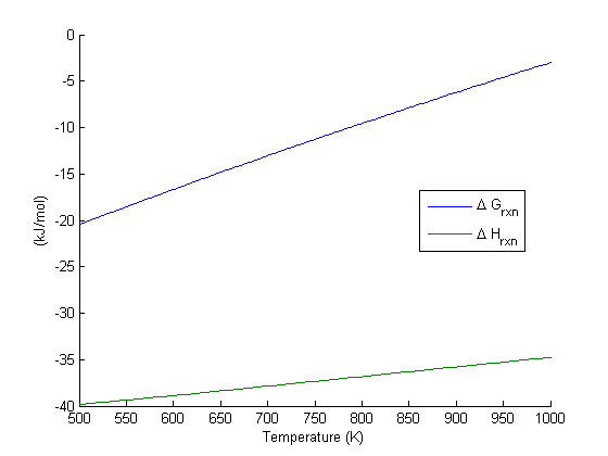
be the extent of reaction, so that $F_i = F_{i,0} + \nu_i \epsilon$. For reactants, $\nu_i$ is negative, and for products, $\nu_i$ is positive. We have to solve for the extent of reaction that satisfies the equilibrium condition.

A = CO
B = H2O
C = H2
D = CO2
Pa0 = 5; Pb0 = 5; Pc0 = 0; Pd0 = 0;  % pressure in atm
R = 0.082;
Temperature = 1000;

% we can estimate the equilibrium like this. We could also calculate it
% using the equations above, but we would have to evaluate each term. Above
% we simple computed a vector of enthalpies, entropies, etc...
K_Temperature = interp1(T,K,Temperature);

% If we let X be fractional conversion then we have $C_A = C_{A0}(1-X)$,
% $C_B = C_{B0}-C_{A0}X$, $C_C = C_{C0}+C_{A0}X$, and $C_D =
% C_{D0}+C_{A0}X$. We also have $K(T) = (C_C C_D)/(C_A C_B)$, which finally
% reduces to $0 = K(T) - Xeq^2/(1-Xeq)^2$ under these conditions.

f = @(X) K_Temperature - X^2/(1-X)^2;

Xeq = fzero(f,[1e-3 0.999]);
sprintf('The equilibrium conversion for these feed conditions is: %1.2f',Xeq)
ans =

The equilibrium conversion for these feed conditions is: 0.55

Compute gas phase pressures of each species

Since there is no change in moles for this reaction, we can directly calculation the pressures from the equilibrium conversion and the initial pressure of gases. you can see there is a slightly higher pressure of H2 and CO2 than the reactants, consistent with the equilibrium constant of about 1.44 at 1000K. At a lower temperature there would be a much higher yield of the products. For example, at 550K the equilibrium constant is about 58, and the pressure of H2 is 4.4 atm due to a much higher equilibrium conversion of 0.88.

P_CO = Pa0*(1-Xeq)
P_H2O = Pa0*(1-Xeq)
P_H2 = Pa0*Xeq
P_CO2 = Pa0*Xeq
P_CO =

    2.2748


P_H2O =

    2.2748


P_H2 =

    2.7252


P_CO2 =

    2.7252

Compare the equilibrium constants

We can compare the equilibrium constant from the Gibbs free energy and the one from the ratio of pressures. They should be the same!

K_Temperature
(P_CO2*P_H2)/(P_CO*P_H2O)
K_Temperature =

    1.4352


ans =

    1.4352

Summary

The NIST Webbook provides a plethora of data for computing thermodynamic properties. It is a little tedious to enter it all into Matlab, and a little tricky to use the data to estimate temperature dependent reaction energies. A limitation of the Webbook is that it does not tell you have the thermodynamic properties change with pressure. Luckily, those changes tend to be small.

% categories: Miscellaneous, nonlinear algebra
% tags: thermodynamics, reaction engineering
Read and Post Comments

Controlling the exit concentration of a CSTR

| categories: miscellaneous | View Comments

Controlling the exit concentration of a CSTR

Controlling the exit concentration of a CSTR

John Kitchin

We examine how to model a CSTR with a controller that varies the volumetric flowrate to control the exit concentration. First we examine a case with no control, then with a simple controller, and then the response of the controller to a change in temperature which modifies the reaction rate.

function main
close all, clc, clear all

V = 100; % volume of CSTR
vo = 20; % volumetric flow rate
Cain = 2;
Ca0 = 2;
tspan = linspace(0,20,20*60); % this is the solution at every second.

    function dCadt = cstr(t,Ca)
        % A -> B
        ra = -0.1*Ca;
        dCadt =  Cain - Ca + ra*V/vo ;
    end

[t,Ca] = ode45(@cstr,tspan,Ca0);

subplot(2,1,1)
plot(t,Ca)
xlabel('Time')
ylabel('C_A')

subplot(2,1,2)
plot(tspan,vo,'b.')
xlabel('time')
ylabel('volumetric flow')

The reactor does not have the desired behavior; the exit concentration is too high. We could simply compute the flow rate required to get the desired exit concentration, but that will only work for this specific set of conditions. If the reactor gets hotter or colder, it will no longer have the desired exit concentration because the reaction rates will change.

Let's implement a controller to actively control the exit concentration by varying the volumetric flow. We will use a simple idea: if the exit concentration is not equal to the desired setpoint, we adjust the volumetric flow by an amount proportional to the difference. We call the proportionality the gain. The choice of the gain factor can have a major impact on the controller. If it is too low, it takes a long time for the system to respond, and if it is too high, the controller may actually be unstable. Here we use a gain that works ok, which we discovered by trial and error. There are ways to determine an optimal behavior that are beyond the scope of this post.

We choose an exit goal of 0.5 mol A/L, corresponding to a conversion of 0.75 for the inlet concentration.

    function vo_in = controller(t,Ca)
        % a simple proportional controller that adjusts  the volumetric
        % flow by an amount proportional to the deviation between the
        % desired and actual exit concentrations.

        setpoint = 0.5;  % desired exit concentration
        error = setpoint - Ca;

        gain = 0.5;
        vo = vo + gain*error;

        % We don't want to allow vo to be negative, and practically it
        % cannot be zero either, since then tau = infinity. Our pump is
        % also limited to a maximum volumetric flow of 40.
        if vo < 0.001;
            vo = 0.001
        elseif vo > 40
            vo = 40;
        end

        % let's plot the volumetric flow to see how it changes everytime
        % this function is called.
        subplot(2,1,2); hold on
        plot(t,vo,'b.')
        vo_in = vo;
    end

    function dCadt = controlled_cstr(t,Ca)
        % A -> B
        ra = -0.1*Ca;

        % the next line sets the volumetric flow.
        vo = controller(t,Ca);
        dCadt =  Cain - Ca + ra*V/vo ;
    end

tspan = linspace(20,40,20*60);
init = Ca(end); % start at the end of the last integration

[t2,Ca2] = ode45(@controlled_cstr,tspan,init);
subplot(2,1,1); hold on
plot(t2,Ca2,'r-')

The controller quickly decreases the volumetric flowrate to increase the residence time, resulting in a decrease in exit concentration. Here you can see the gain is a little too high, because the controller overshoots and the exit concentration, and there are some excursions from the setpoint after that. Those are due to numerical errors in the ODE integration.

Now let's see how the controller responds to a temperature excursion. Suppose the reactor cools down, and the reaction rate is suddenly one half the rate it used to be. The exit concentration will rise, since the reactants are not reacting as fast. The controller should decrease the volumetric flowrate to increase the space time.

    function dCadt = controlled_cstr_temperature(t,Ca)
        % A -> B
        ra = -0.05*Ca;
        vo = controller(t,Ca);
        dCadt =  Cain - Ca + ra*V/vo ;
    end

tspan = linspace(40,60,20*60);
init = Ca2(end); % start at the end of the last integration

[t3,Ca3] = ode45(@controlled_cstr_temperature,tspan,init);

subplot(2,1,1); hold on
plot(t3,Ca3,'k-')

As expected, the concentration initially goes up, then the controller lowers the volumetric flowrate. Also note the controller was able to keep the exit concentration at the setpoint even though the rate of the reaction changed due to the temperature change. There are some notable small deviations from the setpoint near times 47 and 52. These are due to the ODE solver. If you examine the spacing of the points in the volumetric flow graph you will see they are not evenly spaced at 1 sec. That is because the volumetric flow is updated for every call to the ode function, not just at the solution points.

Now that I have tried this, it is clear this is not the best way to model the effect of a controller, because the ODE integrator does some funny things with the time steps. Sometimes the solver appears to take steps back in time to improve the accuracy of the solution, but that is not physically real, and the controller doesn't account for this non-physical behavior. That is why, for example there are excursions from the setpoint after an apparent steady state value is reached in the last example. Maybe this is why everyone uses Simulink for control problems!

end

% categories: Miscellaneous
% tags: control
% post_id = 1460; %delete this line to force new post;
% permaLink = http://matlab.cheme.cmu.edu/2011/11/13/control_cstr-m/;
Read and Post Comments

Unique entries in a vector

| categories: miscellaneous | View Comments

unique_entries

Contents

Unique entries in a vector

John Kitchin

It is surprising how often you need to know only the unique entries in a vector of entries. Matlab provides the unique` to solve these problems. The :command:`unique command returns the sorted unique entries in a vector.

a = [1 1 2 3 4 5 3 5]

unique(a)
a =

     1     1     2     3     4     5     3     5


ans =

     1     2     3     4     5

The unique command also works with cell arrays of strings.

a = {'a'
    'b'
    'abracadabra'
    'b'
    'c'
    'd'
    'b'}

unique(a)
a = 

    'a'
    'b'
    'abracadabra'
    'b'
    'c'
    'd'
    'b'


ans = 

    'a'
    'abracadabra'
    'b'
    'c'
    'd'

There is more!

The unique command has some other features too. check them out:

help unique
 UNIQUE Set unique.
    B = UNIQUE(A) for the array A returns the same values as in A but
    with no repetitions. B will also be sorted. A can be a cell array of
    strings.
 
    UNIQUE(A,'rows') for the matrix A returns the unique rows of A.
 
    [B,I,J] = UNIQUE(...) also returns index vectors I and J such
    that B = A(I) and A = B(J) (or B = A(I,:) and A = B(J,:)).
 
    [B,I,J] = UNIQUE(...,'first') returns the vector I to index the
    first occurrence of each unique value in A.  UNIQUE(...,'last'),
    the default, returns the vector I to index the last occurrence.
 
    See also UNION, INTERSECT, SETDIFF, SETXOR, ISMEMBER, SORT, ISSORTED.

    Overloaded methods:
       cell/unique
       dataset/unique
       RTW.unique
       categorical/unique

    Reference page in Help browser
       doc unique

'done'

% categories: Miscellaneous
ans =

done

Read and Post Comments

Sorting in Matlab

| categories: miscellaneous | View Comments

Sorting in Matlab

Sorting in Matlab

John Kitchin

Occasionally it is important to have sorted data. Matlab provides a sort command with a variety of behaviors that you can use, as well as other related commands.

Contents

Sorting a vector

a = [4 5 1 6 8 3 2]
a =

     4     5     1     6     8     3     2

b_ascending = sort(a)  % default is in ascending order
b_ascending =

     1     2     3     4     5     6     8

You can specify descending order like this

b_descending = sort(a,'descend')
b_descending =

     8     6     5     4     3     2     1

or you can use the command fliplr to reverse the vector sorted in ascending order.

fliplr(b_ascending)
ans =

     8     6     5     4     3     2     1

Sorting a matrix

If you have data organized in a matrix, you need to be aware of what sorting means. You can sort rows or columns!

a = [5 1 5 4 3
     0 7 1 2 3];

 sort(a)
ans =

     0     1     1     2     3
     5     7     5     4     3

sort works columnwise by default. If you wanted the rows sorted, you need:

sort(a,2)
ans =

     1     3     4     5     5
     0     1     2     3     7

How can you remember that? Indexing in Matlab is (row,column). This notation means sort along the columns. In other words, the row is fixed, and you sort along the columns.

Where would this ever come up? We use it in cmu.der.derc to ensure the x-values are in ascending order before we compute the derivative! It is also convenient to sort data before plotting it if you connect the datapoints by lines.

x = [9 1 2 5 6 7];
y = sin(x);

plot(x,y)

Note how the lines cross each other. That is visually distracting, and simply an artifact of the ordering of the points. We can use an extra feature of sort to sort x and y, so that x is sorted in ascending order, and we use the change in the order of x to get the corresponding changes in y. This is a handy trick!

[X I] = sort(x);
Y = y(I);
plot(X,Y)
'done'

% categories: Miscellaneous
ans =

done

Read and Post Comments

« Previous Page -- Next Page »